Chi-squared Test

In practice, there are two possible Chi-squared tests:

• A chi-square goodness of fit test determines if a sample data matches a population.
• A chi-square test for independence compares two variables in a contingency table to see if they are related.

In general, we consider the Chi-squared test to see whether distributions of categorical variables differ from each another.

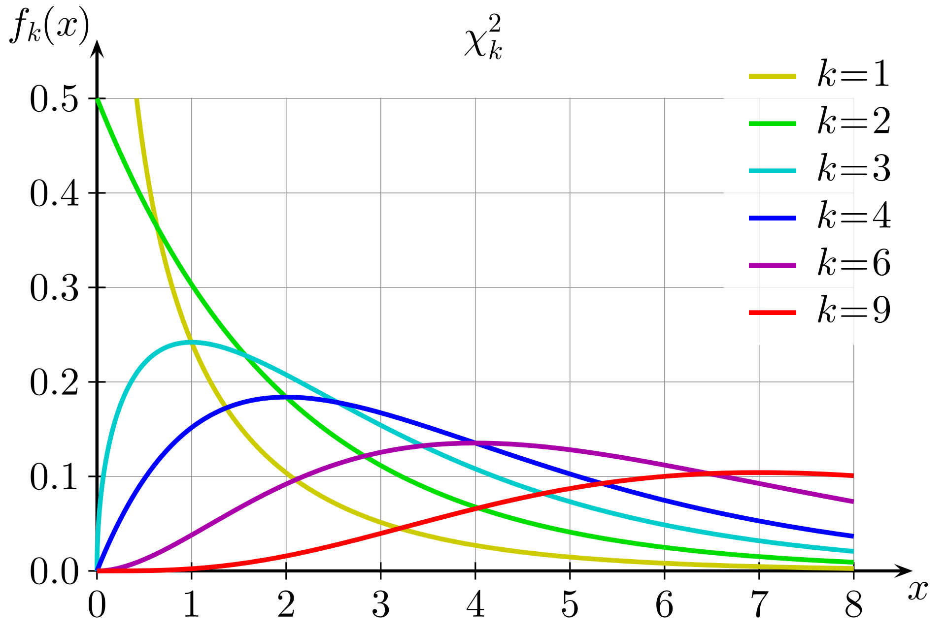
1. Defintion: Chi-squared Distribution

If $Z_1, ..., Z_k$ are independent, standard normal random variables, then the sum of their squares,

$$\begin{align} Q\ =\sum _{i=1}^{k}Z_{i}^{2}, \end{align}$$

is distributed according to the chi-squared distribution with k degrees of freedom. This is usually denoted as

$$\begin{align} Q\ \sim \ \chi ^{2}(k) \end{align}$$

The chi-squared distribution has one parameter: a positive integer k that specifies the number of degrees of freedom (the number of $Z_i$’s).

The term ‘chi square’ (pronounced with a hard ‘ch’) is used because the Greek letter $\chi$ is used to define this distribution. It will be seen that the elements on which this distribution is based are squared, so that the symbol $\chi^2$ is used to denote the distribution.

2. Chi-squared Statistics

For both the goodness of fit test and the test of independence, the Chi-squared statistic is the same. For both of these tests, all the categories into which the data have been divided are used. The data obtained from the sample are referred to as the observed numbers of cases. These are the frequencies of occurrence for each category into which the data have been grouped. In the Chi-squared tests, the null hypothesis makes a statement concerning how many cases are to be expected in each category if this hypothesis is correct. The Chi-squared test is based on the difference between the observed and the expected values for each category. The chi square statistic is defined as

$$\begin{align} \chi^2 = \sum \frac{(O_i - E_i)^2}{E_i}\end{align}$$

where $O_i$ is the observed number of cases in category i, and $E_i$ is the expected number of cases in category i. This Chi-squared statistic is obtained by calculating the difference between the observed number of cases and the expected number of cases in each category. This difference is squared and divided by the expected number of cases in that category. These values are then added for all the categories, and the total is referred to as the Chi-squared statistic.

3. Approximation

According to the work of Pearson and many afterwards, under the circumstance of the null hypothesis being correct (i.e. the observed are part of the large population satisfying the expected statistical behavior), as $n \rightarrow \infty$, the limiting distribution of the quantity given below is the $\chi^2$-distribution. In practice, the condition in which the Chi-square statistic is approximated by the theoretical Chi-squared distribution, is that the sample size is reasonably large and the rough rule of thumb concerning sample size is that there should be at least 5 expected cases per category.

4. Examples

Example 1. There are four blood types (ABO system). It is believed that 34%, 15%, 23% and 28% of people have blood type A, B, AB and O respectively. The blood samples of 100 students were collected: A(12), B(56), AB(2), O(30). Test if the collected blood sample contradicts the previous belief. Solution. The null hypothesis would be

$$\begin{align} H_0:p_A=0.34, p_B=0.15,p_{AB}=0.23,p_O=0.28. \end{align}$$

We compute the Chi-squared test statistic as follows:

$$\begin{align} \chi^2 & = (12-34)^2/34+(56-15)^2/15+ (2-23)^2/23+(30-28)^2/28 \\ & = 145.6187 \end{align}$$

Since the corresponding $P$-value is almost 0, we reject $H_0$.

Example 2. The number of accidents $X$ per week at an intersection was checked for 50 weeks: 32weeks with no accident, 12 weeks with 1 accident, 6 weeks with 2 accidents. Test if $X$ follows a Poission distribution.

Solution. The null hypothesis is given by

$$\begin{align} H_0: P(X=x)=\lambda^x e^{-\lambda}/x! \end{align}$$

for all $x=0,1,2,\cdots$. Since $\lambda$ unknown, we estimate it with MLE.

$$\begin{align} \hat \lambda = \bar x =(12+2\times6)/50=0.48. \end{align}$$

Define three categories by $X=0$ , $X=1$, and $X \geq 2$. The expected probabilities are estimated to give $\hat p_1 =0.619$, $\hat p_2=0.297$, and $\hat p_3 = 1-\hat p_1 -\hat p_2=0.084$. Then the test statistic $\chi^2 \sim \chi^2_1$ (the additional degree of freedom is lost due to the estimation of $\lambda$). $\chi^2=1.354$ and the $P$-value would be 0.25. We do not reject $H_0$.

4. Conclusion

• A very small chi square test statistic means that your observed data fits your expected data extremely well. In other words, there is a relationship.

• A very large chi square test statistic means that the data does not fit very well. In other words, there isn’t a relationship.

5. Application

For an interesting application of Chi-squared test in relation to Benford’s law and checking authenticity of any numerical data like presidential votes and company revenue, please see my jupyter notebook.