Because of the NFL (No Free Lunch) Theorem, it seems that machine learning is doomed to fail. With the introduction of statistical tools, we learned that when the random sample size is large enough and the number of hypothesis is reasonably small, then machine learning is viable. In this part, we will rigorously disucss the core problem of when can a machine learn.
Training versus Testing
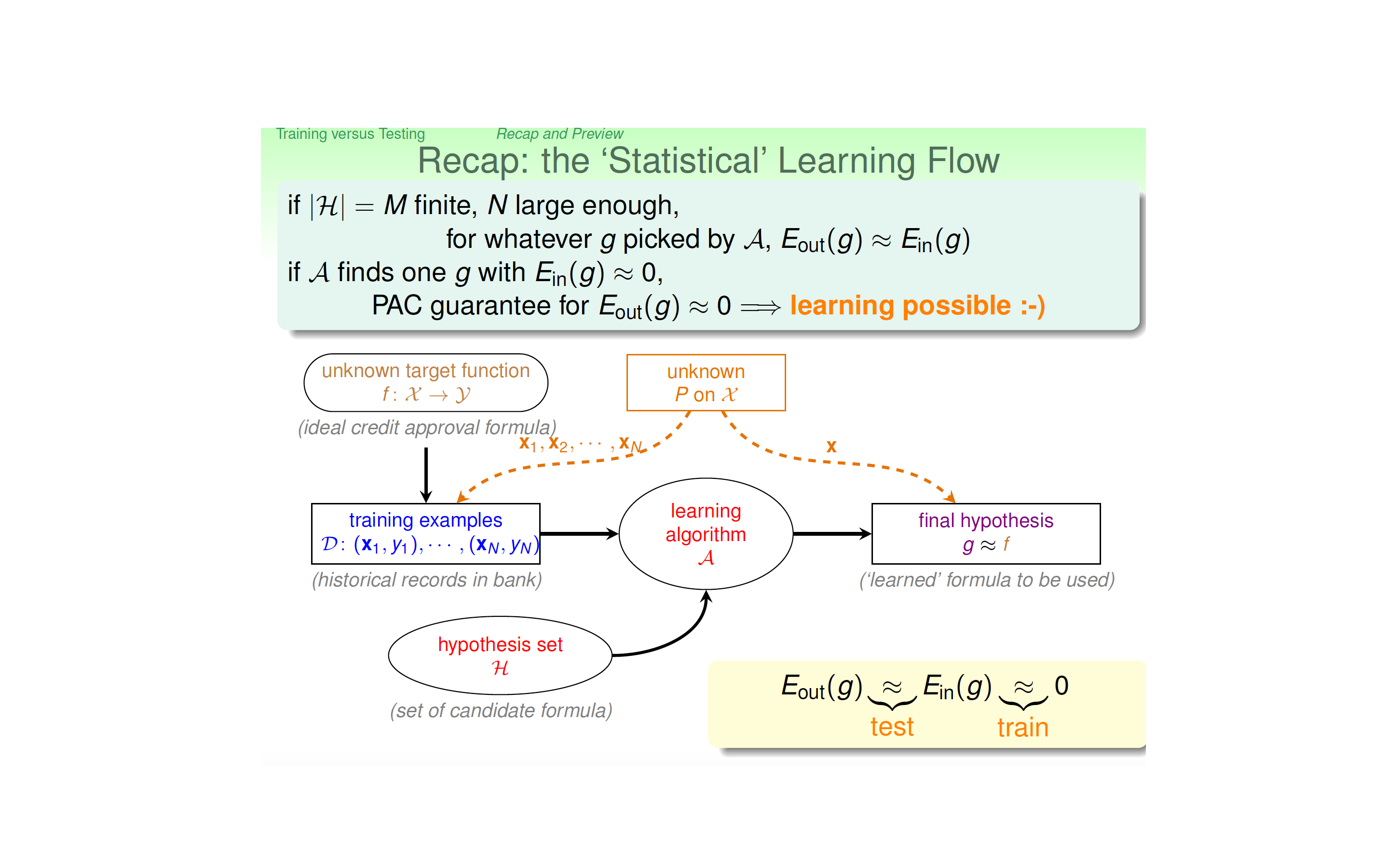
Let us look at the following flow chart of supervised learning:

In the above “statistical” learning flow, we need that the training dataset and the test dataset all obey the same population distribution, this is the fundamental reason why machine can learn. Also, we require that the training dataset is relatively large and the number of hypothesis is reasonably bounded. Therefore, according to the Hoeffding inequality, we can show that our algorithm can be generalized well. With good training, we can therefore get our final model \(g \approx f\), the latter being our noisy target.
Generalization Error
We have discussed how the value of \(E_{in}\) does not always generalize to a similar value of \(E_{out}\). Generalization is a key issue in learning. One can define the generalization error as the discrepancy between \(E_{in}\) and \(E_{out}\)· By the Hoeffding Inequality as discussed before, we can characterize the generalization error with a probabilistic bound,
\[\begin{align} \mathbb{P}[\lvert E_{in}(g) - E_{out}(g) \rvert > \epsilon] \leq 2 |\mathcal{H}| e^{-2n\epsilon^2} \end{align}\]for any \(\epsilon > 0\). Here the factor \(\mathcal{H}\) is due to simple set theoretic consideration and its explanation can be found on p41 in Learning from data.
Effective Number of Hypotheses
We now introduce the growth function, the quantity that will formalize the effective number of hypotheses and will use it to replace \(\lvert \mathcal{H}\rvert\) in the above inquality. It is a combinatorial quantity that captures how different the hypotheses in \(\mathcal{H}\) are and its definition is given by
\[\begin{align} m_{\mathcal{H}}(n) = \max_{X_1, \cdots, X_n \in \mathcal{X}} \lvert \mathcal{H}(X_1, \cdots, X_n)\rvert \end{align}\]where \(\lvert \rvert\) denotes the cardinality (number of elements) of a set and \(\mathcal{H}(X_1, \cdots, X_n)\) denotes the space of vectors generated by \(\mathcal{H}\) on the specified data set inside the total space of data \(\mathcal{X}\). In general, we have
\[\begin{align} m_{\mathcal{H}}(n) \leq 2^{n} \end{align}\]Example

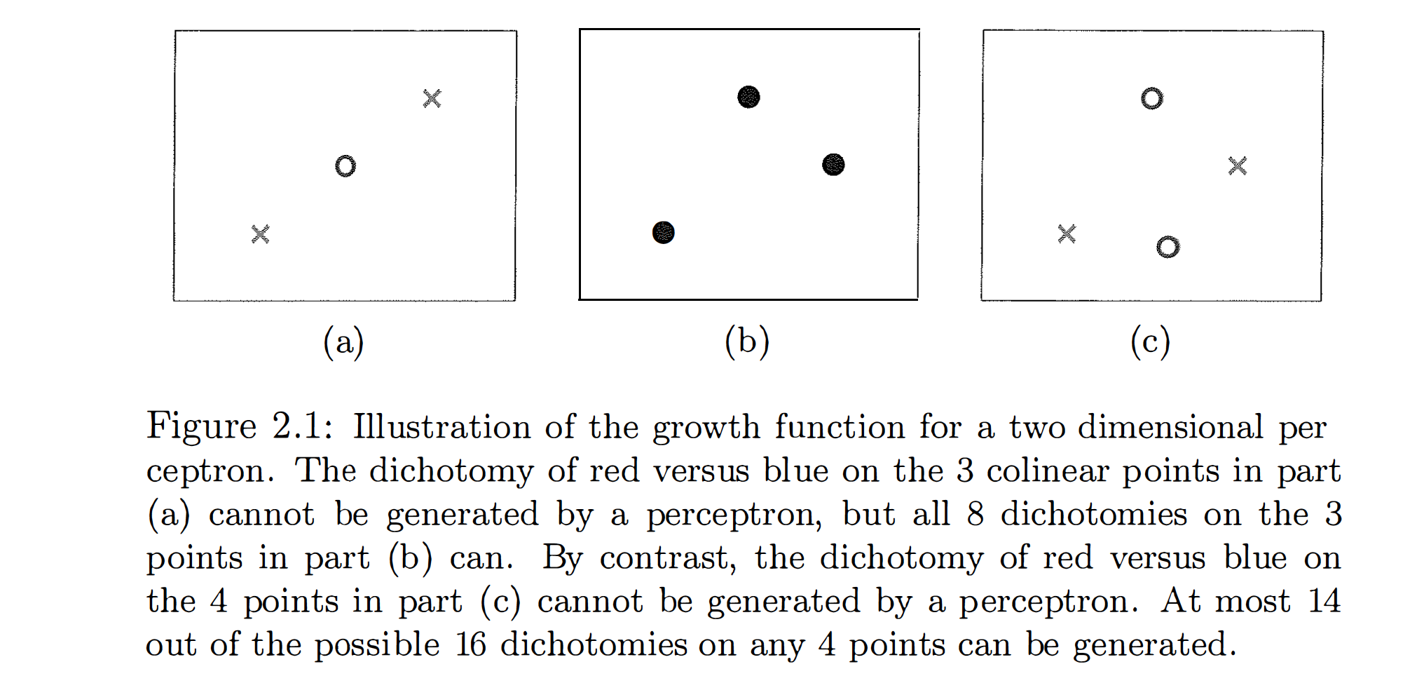
If no data set of size k can be shattered by \(\mathcal{H}\), then k is said to be a break point for \(\mathcal{H}\). If k is a break point, then \(m_{\mathcal{H}}(k) < 2^k\).
Theorem: If \(m_{\mathcal{H}}(k) < 2^k\) for some value k, then
\[\begin{align} m_{\mathcal{H}}(k) \leq \sum_{i=0}^{k-1} {n \choose i} \end{align}\]for all N. The RHS is polynomial in N of degree k-1. The implication of this theorem is that if \(\mathcal{H}\) has a break point, we have what we want to ensure good generalization; a polynomial bound on \(m_{\mathcal{H}}(k)\), since then the discrepency betweent the in-sample and out-sample error diminishes as sample size increase.