Given a training dataset \(\mathcal{D}\) out of a larger population data and suppose our goal is to learn a “noisy” target function \(f\) on the popultation from the training data. In supervised learning, we usually take the following strategy:

• Pick some class of functions \(f(x)\) (decision trees, linear functions, etc.)
• Pick some loss function, measuring how we would like \(f(x)\) to perform on test data.
• Fit \(f(x)\) so that it has a good average loss on training data. (Perhaps using cross- validation to regularize.)

What is missing here is a proof that the performance on training data is indicative of performance on test data. Does the data set \(\mathcal{D}\) tell us anything outside of \(\mathcal{D}\) that we didn’t know before? We intuitively know that the more “powerful” the class of functions is, the more training data we will tend to need, but we have not made the definition of “powerful”, nor this relationship precise.

In this note, we will study some of the most basic ways of characterizing the “power” of a set of functions.

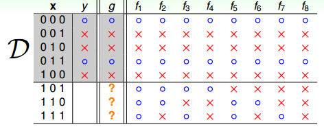
Let us consider the following example: suppose we want to learn a Boolean target function over a three-dimensional input space \(X = \{0, 1\}^3\)，while the training dataset \(\mathcal{D}\) contains 5 out of all 8 possible outputs.

Therefore，there exist 8 possible candidate hypothesis for \(f\), which all classify the 5 training data correctly, but on the remaining 3 test data，their performance differ greatly. How do we know which hypothesis to learn given one of them is the target function, and remember that it is the hypothesis’ performance on the test data that we care.

No Free Lunch Theorem

The NFLT states that under the following conditions:

• The search space the optimiser iterates through will be finite;
• The space of possible cost values will also be finite;

any one algorithm that searches for an optimal cost or fitness solution is not universally superior to any other algorithm.

Probability to Rescue

The key observation here is that, we will want our observations be random, which will allow us to believe that our observations are representative of the larger population.

Hoeffding’s inequality:

Suppose that \(X_1,...,X_n\) are random independent identically distributed random variables satisfying that \(0 \leq X_i \leq 1\) and \(\mathbb{E}[X] = \mu\). Then for any \(\epsilon >0\),

\[\begin{align} \mathbb{P}(\lVert \frac{1}{n} \sum X_i − \mu \rVert \geq \epsilon) \leq 2 \text{exp}\big( - {2n \epsilon^2}\big) \end{align}\]

where \(\mathbb{P}(\cdot)\) denotes the probability of an event.

The intuition for this result is very simple. We have a bunch of variables \(Z_i\). We know that when we average a bunch of them up, we should usually get something close to the expected value. Hoeffding quantifies “usually” and “close” for us.

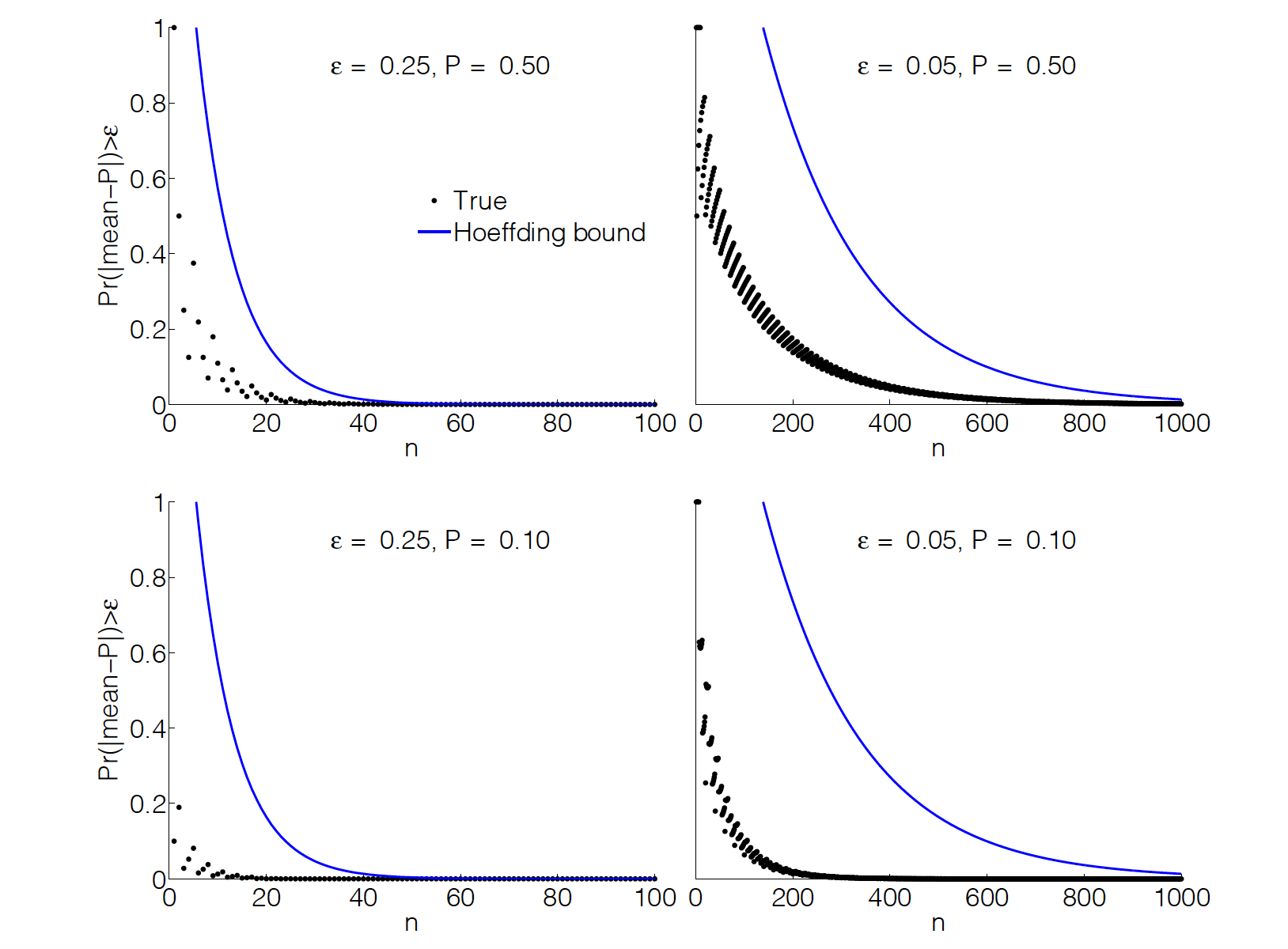
The following examples compare Hoeffding’s inequality to the true probability of deviating from the mean by more than for binomial distributed variables, with \(E[Z] = \mu\). For \(\mu = 1/2\) the bound is not bad. However, for \(\mu = 1/10\) it is not good at all. What is happening is that Hoeffding’s inequality does not make use of any properties of the distribution, such as its mean or variance. In a way, this is great, since we can calculate it just from n and \(\epsilon\). The price we pay for this generality is that some distributions will converge to their means much faster than Hoeffding is capable of knowing.

Another form of Hoeffding’s inequality of the following.

Let \(\delta = 2 \text{exp}(-2n\epsilon^2)\) and suppose we choose

\[\begin{align} n \geq \frac{1}{2\epsilon^2} \text{log}\frac{2}{\delta} \end{align}\]

Then, with probability at least \(1-\delta\), the difference between the empirical mean \(\frac{1}{n} \sum Z_i\) and the true mean \(\mathbb{E}[Z]\) is at most \(\epsilon\).

To understand this second form, we can think of setting two “slop” param- eters:

• The “accuracy” \(\epsilon\) says how far we are willing to allow the empirical mean to be from the true mean.
• The “confidence” \(\delta\) says what probability we are willing to allow of “failure”. (That is, a deviation larger than \(\epsilon\))

If we choose these two parameters, the second form of the above inequality quantifies how much it will “cost” in terms of samples.

When applied to the important special case of identically distributed Bernoulli random variables \(X_i\) with sample mean \(\nu\), the above inequality specialize to

\[\begin{align} \mathbb{P}(\lVert \nu − \mu \rVert \geq \epsilon) \leq 2 \text{exp}\big( -{2n \epsilon^2}\big) \end{align}\]

which says that as the sample size n grows, it becomes exponentially unlikely that v will deviate from \(\mu\) by more than our ‘tolerance’ \(\epsilon\). The proof of the Hoeffding theorem can be found here.

Relation to Learning Theory

Let us consider an entire hypothesis set \(\mathcal{H}\) used to approximate our noisy target \(f\) and assume for the moment that \(\mathcal{H}\) has a finite number of hypotheses. Given any \(g \in \mathcal{H}\), we will denote the error rate within the sample, called the in-sample error, by

\[\begin{align} E_{in}(g) & = (\text{fraction of}\ \mathcal{D}\ \text{where}\ f\ \text{and}\ g \ \text{disagree}) \\ & = \frac{1}{n} \sum \lVert f(x_i) \neq g(x_i) \rVert \end{align}\]

where \(\lVert \text{statement} \rVert = 1\) if the statement is true, and \(= 0\) if the statement is false. In the same way, we define the out-of-sample error

\[\begin{align} E_{out}(g) = \mathbb{P}[f(X_i) \neq g(X_i)] \end{align}\]

What Hoeffding theorem is saying is that we can probably almost correctly make \(E_{in}(g)\) sufficiently close to \(E_{out}(g)\), which makes learning feasibile. You may be tempted to do the following to approximate \(f\):

• Input the set of classifiers (hypothesis) \(\mathcal{H}\);
• Draw \(n \geq \frac{1}{2 \epsilon^2}\text{log}\frac{2}{\delta}\) samples;
• Output \(g^* = \min_{g \in \mathcal{H}} E_{in}(g)\).

We might be tempted to conclude that since \(E_{in}(g)\) is close to \(E_{out}(g)\) with high probability for all g, the output \(g^*\) should be close to the best class. Trouble is, it isn’t true!

One way of looking at the previous results is this: for any given classifier, there aren’t too many “bad” training sets for which the empirical risk is far off from the true risk. However, different classifiers can have different bad training sets. If we have 100 classifiers, and each of them is inaccurate on 1% of training sets, it is possible that we always have at least one such that the empirical risk and true risk are far off. (On the other hand, it is possible that the bad training sets do overlap. In practice, this does seem to happen to some degree, and is probably partially responsible for the fact that learning algorithms generalize better in practice than these type of bounds can prove.)

The way to combat this is to make the risk of each particular classifier being off really small. If we have 100 classifiers, and want only a 1% chance of failure, we limit the probability of failure of each to 0.01%. Or, if we want an overall probability of failure of \(\delta\), we make sure that each individual classifer can only fail with probability \(\delta/\lvert \mathcal{H} \rvert\). Plugging this into our previous result, we have

Theorem: with probability \(1 - \delta\), for all \(g \in \mathcal{H}\) simultaneously

\[\begin{align} \lvert E_{in}(g) - E_{out}(g)\rvert \leq \sqrt{\frac{1}{2n} \text{log} \frac{2\lvert \mathcal{H} \rvert}{\delta}} \end{align}\]

The remaining question is if we can make \(E_{in}(g)\) small, which will be answered by the various learning algorithms to be introduced.

Complexity of the space of all hypothesis \(\mathcal{H}\)

If the size of hypotheses set \(\mathcal{H}\) goes up, we run more risk that \(E_{in}(g)\) will be a poor estimator of \(E_{out}(g)\) according to the Hoeffding inequality. Thus \(\lvert \mathcal{H}\rvert\) can be thought of as a measure of the ‘complexity’ of \(\mathcal{H}\). If we want an affirmative answer to the first question, we need to keep \(\lvert \mathcal{H}\rvert\) in check. However, if we want an affirmative answer to the second question, we stand a better chance if \(\mathcal{H}\) is more complex, since g has to come from \(\mathcal{H}\). So, a more complex \(\mathcal{H}\) gives us more flexibility in finding some g that fits the data well, leading to small \(E_{in}(g)\). This tradeoff in the complexity of \(\mathcal{H}\) is a major theme in learning theory.

VC-dimension and Infinite Hypothesis Space

With probability \(1-\delta\), for all \(g \in \mathcal{H}\) simultaneously,

\[\begin{align} E_{in}(g) \leq E_{out}(g) + \sqrt{\frac{VC[\mathcal{H}]}{n}(\text{log}\frac{n}{VC[\mathcal{H}]} + \text{log}2e) + \frac{1}{n}\text{log}\frac{4}{\delta}} \end{align}\]

Where \(VC[\mathcal{H}]\) is the VC-dimension of the set \(\mathcal{H}\), which is defined as the size of the largest data set \(\mathcal{D}\) that can be shattered by \(\mathcal{H}\).

Error and Noise

Learning is not expected to replicate the target function perfectly. The final hypothesis g is only an approximation of f. To quantify how well g approximates f, we need to define an error measure that quantifies how far we are from the target.

The choice of an error measure affects the outcome of the learning process. Different error measures may lead to different choices of the final hypothesis, even if the target and the data are the same, since the value of a particular error measure may be small while the value of another error measure in the same situation is large. Therefore, which error measure we use has consequences for what we learn.

One can think of a noisy target as a deterministic target plus added noise. If y is real-valued for example, one can take the expected value of y given x to be the deterministic \(f(x)\), and consider \(y - f(x)\) as pure noise that is added to f .

Reference

Introduction to Statistical Learning Theory, Bousquet, Boucheron, Lugosi, Advanced Lectures on Machine Learning Lecture Notes in Artificial Intelligence, 2004