A perceptron is a linear (binary) classifier on the training dataset \(\{x_i, y_i\}\) where \(y_i\) takes value in \(\{-1, +1\}.\)

The Linear Separability Assumption

For a perceptron classifier to work, we need the data set to be linearly separable. As you may know, two sets are linearly separable if and only if their convex hull has no intersection. Famous example of a simple non-linearly separable data set, the XOR problem is given by Minsky in 1969, which led to invention of multi-layer networks. To check the linear separable condition, we can apply the convex hull algorithm or to use the linear SVM to see if the corresponding error vanishes.

The Classifier

We composite the sign function with the linear regression model to get

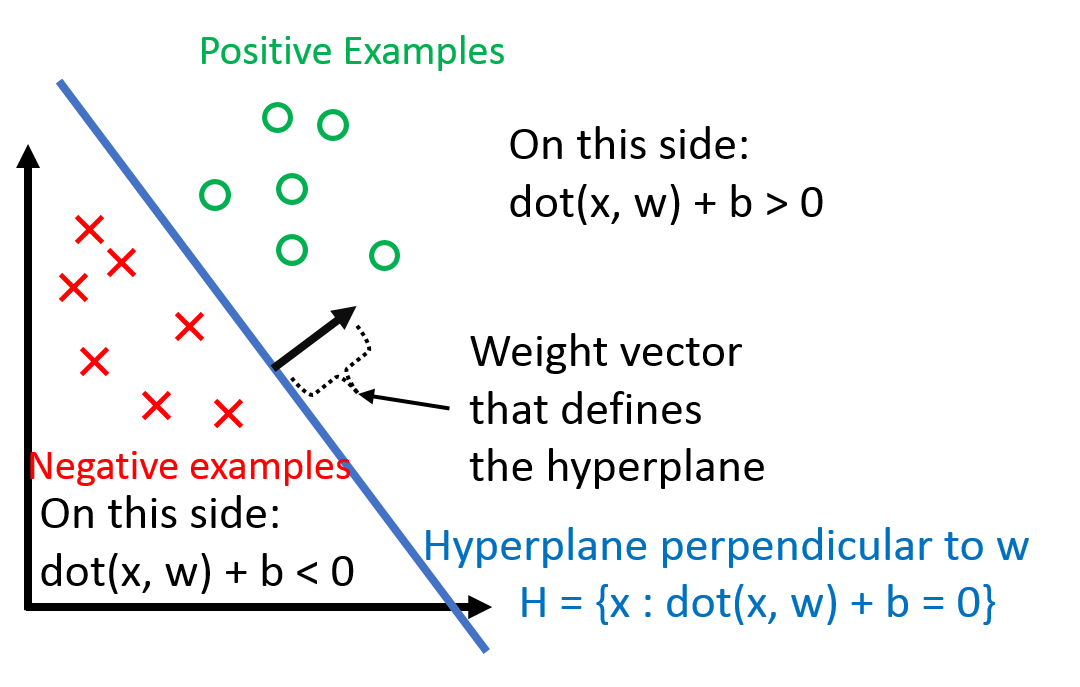
\[\begin{align} h(x_i) = \text{sign}(\mathbf{w}^{T}x_i + b) \end{align}\]

where b is the threshold term (intuitively the y-intercept in 2-D). See the following picture for an intuitive understanding of the perceptron model:

As dealing with b can be a pain, we ‘absorb’ it into the weight vector \(\mathbf{w}\) by adding one additional constant dimension. Under this convention,

\[\begin{align*} \mathbf{x}_i \hspace{0.1in} \text{becomes} \hspace{0.1in} \begin{bmatrix} \mathbf{x}_i \\ 1 \end{bmatrix} \\ \mathbf{w} \hspace{0.1in} \text{becomes} \hspace{0.1in} \begin{bmatrix} \mathbf{w} \\ b \end{bmatrix} \\ \end{align*}\]

with these new notations, we simplify as

\[\begin{align} h(\mathbf{x}_i) = \textrm{sign}(\mathbf{w}^\top \mathbf{x}) \end{align}\]

Geometrically speaking, any hyperplane given by the weight vector \(\mathbf{w}\) is an eligible perceptron and therefore there are infinitely many possible choices. How dow we choose one based on the training data set \(\{(x_i, y_i)\}\). A key obervation is that

\[\begin{align} y_i(\mathbf{w}^\top \mathbf{x}_i) > 0 \Longleftrightarrow \mathbf{x}_i \hspace{0.1in} \text{is classified correctly} \end{align}\]

where ‘classified correctly’ means that \(x_i\) is on the correct side of the hyperplane defined by the weight vector \(\mathbf{w}\). Also, note that the left side depends on \(y_i \in \{−1,+1\}\) (it wouldn’t work for \(yi \in \{0,+1\}\)).

The Perceptron Learning Algorithm

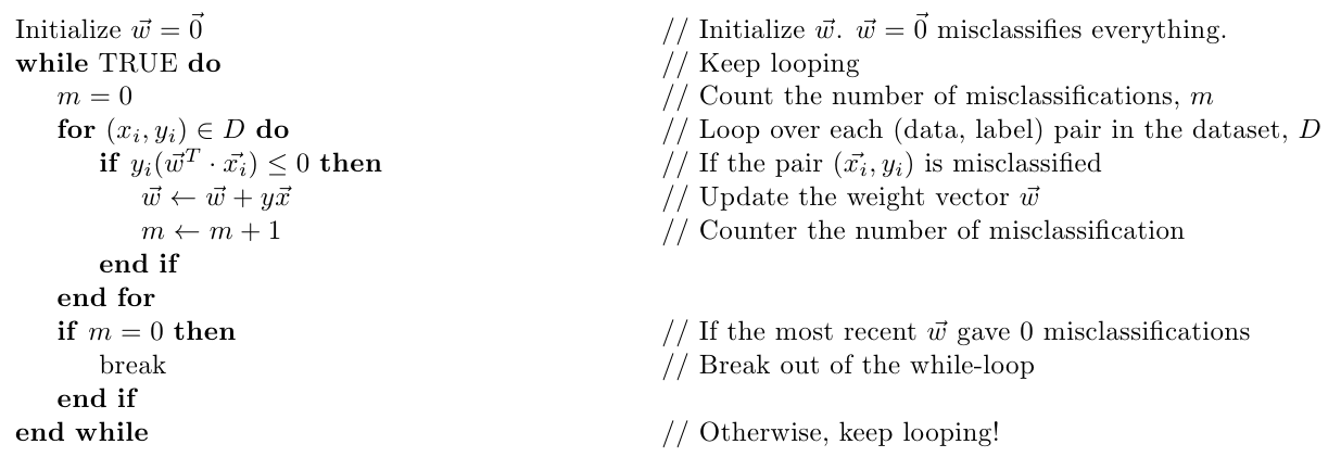
Now that we know what the w is supposed to do (defining a hyperplane the separates the data), let’s look at how we can get such w:

Intuitively, we have

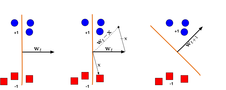
(Left:) The hyperplane defined by \(\mathbf{w}_t\) misclassifies one red (-1) and one blue (+1) point. (Middle:) The red point x is chosen and used for an update. Because its label is -1 we need to subtract x from \(\mathbf{w}_t\). (Right:) The udpated hyperplane \(\mathbf{w}_{t+1}\) = \(\mathbf{w}_t\) − \(\mathbf{x}\) separates the two classes and the Perceptron algorithm has converged.

Convergence Theroem of the Perceptron Algorithm

The theorem states that for any finite set of linearly separable labeled examples, the perceptron learning algorithm will halt after a finite number of iterations. In other words, after a finite number of iterations, the algorithm yields a vector \(\mathbb{w}\) that classifies perfectly all the examples.

We refer the interested reader to the rigourous proof of the convergence theorem.

More About Perceptron Learning Algorithm

• Pro: simple to implement, fast, works in any dimension.
• Con: linear separable unknown a priori, halting time unknown which depends on the how “separated” the training data is.
• If the data set is not linear separable and if we relax the condition to find a line which minimize the number of mistakes \(\{ y_i \neq sign(\mathbf{w}^T\mathbf{x_i})\}.\) This problem is NP-hard to solve, unfortunately.
• The alternate solution is to hold somewhat the “best” weight in a pocket.